Analysis options
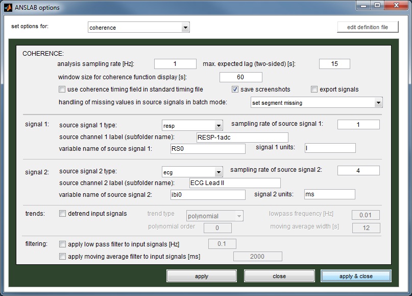
In the ANSLAB options various different settings regarding the analysis can be adjusted:
- Sampling rate to be used for analysis (the source signals are upsampled or downsampled accordingly).
- The maximum expected two-sided lag between the source signals (e.g. setting this value to 10 means
that the maximum expected lag between the signals lies between -10s and +10s).
- The size of the coherence function display (again two-sided). This parameter has no impact on the
analysis as it is only used for displaying the analysis results.
- For each of the two source signals the type (e.g. ecg), the sampling rate (e.g. 4 Hz), the source signal
folder within the ANSLAB study folder (e.g. ECG), the name of the variable to use for the analysis (e.g. ibi0), and the signal unit
can be specified (e.g. ms in case of ibi0).
In addition, the option 'export signals' allows to export the source signals as they are used into a text file.
This text file is stored in the same directory as the result file from the analysis.
The sampling rate of the data stored in this text file corresponds to the analysis sampling rate. The signal parts
stored in the exported files do not correspond to the whole signal, but to the timing segments used for the analysis.
Note: to avoid using wrong source signal sampling rates, ANSLAB aims to automatically detect the sampling rates
used in the source signal files (i.e. ANSLAB looks for the variable 'ep' in the respective mat-files). If the
sampling rate for a source signal can not be determined, ANSLAB uses the value entered in the options dialog for the respective source signal.
In addition to these settings, one might also enable detrending for the source signals in order to compensate
for signal drifts. Or, if the source signals are noisy, one might also enable lowpass filtering for the source signals or decide
to apply a moving average filter to the input signals.
Since during the scoring process, one might choose between different methods to handle missing values in the source signals, the options
dialog also offers the possibility to set the default method to be used in batch mode.
For the configuration example below, ANSLAB will try to find the variable ibi0 in the 'ECG'-subfolder within the 'ecg'-subfolder
and the variable DWV in the 'DW'-subfolder within the 'temp'-subfolder of the study folder. Furthermore, ANSLAB loads the data,
assuming that the respective variables are sampled with the sampling rates given (if the sampling rates can not be determined automatically).
Important: in order to obtain meaningful results, ensure that the source signals selected for the coherence analysis
are sampled evenly. That is, while both signals may have been sampled at different sampling rates, both signals
must have been sampled evenly at the respective sampling rates.
Hint: if you want to compute the coherence between an ANSLAB variable and a variable not produced by ANSLAB, just create
an arbitrarily named subfolder within an ANSLAB analysis subfolder (inside the study folder). Just ensure that the name
of the subfolder does not interfere with an ANSLAB result folder (it is recommended to use an analysis subfolder which
is not used for the current study). Inside the created subfolder place a mat-file containing the variable not produced by ANSLAB.
To ensure that ANSLAB is able to find the mat-file, the naming convention of ANSLAB must be met. If, for example, the raw-file is
named 'TEX00101.ACQ' the mat-file must have the name 'TEX0010100.mat'.
In the example configuration above a mat-file containing the variable 'DWV' (dial-wheel data) has been placed inside a subfolder 'DW' inside the
'temp' folder in the study folder.
[
Top]
Timing files
Before loading the source signals, ANSLAB verfies that a timing file for the coherence analysis is present
next to the raw file. If no timing-file is found, the analysis will be aborted.
The coherence timing file has the same structure as a standard ANSLAB timing file (see
Segmentation & timing).
The only difference is the file extension which must be used. While a standard timing file has the file extension '.m' (e.g. 'TEX00101.m'), the
coherence timing file must have the file extension '.coherence.m' (e.g. 'TEX00101.coherence.m').
[
Top]
Analysis procedure
General procedure
Similar to the cross-spectral analysis, the coherence analysis is started by selecting the raw data file to be processed.
ANSLAB then loads the specified variables from the result files for the raw file selected (from the source signal folders set
in the options). This is followed by resampling the signals if necessary (i.e. if the analysis sampling rate differs
from the sampling rates of the source signals).
ANSLAB then jumps to the first interval defined in the timing file and displays
the two source signals inside the interval and the analysis results for the interval (see example screenshot below).

The result graph contains the following elements:
- the cross-correlation between the source signals over different values
for the time lag (blue curve).
- indicators for the max. expected two-sided lag as set in the options (blue dashed vertical lines).
- a gray, vertical line, showing the position for a lag of zero seconds.
- a gray, solid, horizontal line, showing the line of zero correlation.
- a gray, dashed, horizontal line, showing the maximum correlation found for different time lag values.
- a magenta, vertical line, indicating the time lag for the maximum correlation between the signals.

In addition, the title of the result graph shows the optimal lag value along with the respective correlation-coefficient and
the correlation at lag zero.
Note that when setting the analysis type to 'coherence', the 'dynamic'-section changes to show the scoring controls
(see right image).
Use the buttons
accept and
set missing
to jump from interval to interval and decide wether the results for
the current interval are valid or not. The different buttons in the 'dynamic'-section have the following meanings:
| accept |
saves the results for the current interval and switches to the next
interval |
| set missing |
will set the results for the current interval to NaN (not a number) and
switch to the next interval |
| <<< |
will go back to the previous interval |
| lin. interp. |
will linearly interpolate missing values in the source signals for the current segment and restart
the coherence analysis for the current segment
(explained in more detail below) |
| remove gaps |
will remove parts of the source signals for the current segment which correspond to missing values
(from both source signals) and restart the coherence analysis for the current segment
(explained in more detail below) |
| restart |
will switch to the first interval (i.e. the scoring starts from scratch) |
In addition, one might jump directly to an interval by entering the respective interval number
into the field next to
jump to segment. After hitting enter, ANSLAB saves the results for the current interval and
then switches to the desired interval.
Note: to avoid missing data when directly jumping to intervals, ANSLAB permits to jump only to
already scored intervals or at most one interval after the last already scored interval.
Once all intervals have been
scored, ANSLAB shows a summary of the analysis results for all intervals.

To save the analysis results for later use, click on the button
Save reduced data which
shows up when the last interval has been scored. The according mat-file will be saved in the currently active study folder (in the
subfolder 'coherence'). Since different combinations of source signals may be analyzed for a certain study, ANSLAB creates a
subfolder within the folder 'coherence' which is named after the signals used for the analysis (e.g. subfolder 'ibi0_DWV' for the
configuration as used in the example above).
[
Top]
Dealing with missing data in source signals
Sometimes a source signal will contain missing values (i.e. NaN-values). This could, for example, be the result
of editing ECG data and excluding parts of the signal. As a consequence, the resulting IBI data will contain missing values.
Performing the coherence analysis on such signals without preparing the signals properly will certainly lead to
invalid results.
Therefore, the coherence module offers different ways to handle such signal parts. The user is able
to select the respective method for each segment separately by using the buttons
lin. interp. and
remove gaps in the 'dynamic'-section (as already indicated above).
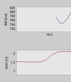
The following image shows an example for a segment in which a source signal contains missing values:

From this image one notices that the first signal has missing data at the beginning of the segment.
Hence, initially no coherence analysis is performed. Instead a message will be shown in the result graph,
indicating that a method to deal with this situation has to be chosen. The user has now the following
options to choose from:
- Set segment to missing
By pressing set missing the results for the current segments are all
set to NaN and the scoring processing continues with the next segment. When no coherence
analysis results have been computed yet due to missing data, hitting accept has the same
effect.
- Use linear interpolation
By pressing lin. interp. all missing parts of the source signals are
interpolated linearly and the coherence analysis results are (re)computed. The parts of the source signals
which previously contained missing values are now shown in red after the interpolation (to be
able to see the effect of the interpolation).
If the result after the interpolation should be accepted, hit accept. Otherwise, either
select another method to deal with missing data or set the segment to missing by hitting set missing.
- Remove gaps from source signals
By hitting remove gaps all gaps will be located in both signals within the current segment.
All signal parts corresponding to a gap in one of the source signals will then be removed
from both signals and the coherence analysis results are (re)computed.
The parts of the source signals which correspond to removed gaps will be indicated
by a red dotted line in both source signal graphs (to be able to see which parts are removed for the coherence analysis).
If the result after gap removal should be accepted, hit accept. Otherwise, either
select another method to deal with missing data or set the segment to missing by hitting set missing.
Important: if the 'export signals'-option is enabled the signals are usually
exported in chronological order without any gaps inside the respective segments. However, if gaps are removed
in order to handle missing values, the same gaps will be present in the exported data.
Note: in batch mode the method specified in the options is used automatically. But there
might be situations in which the selected method will fail and the coherence module will fall back to set the respective segments
to missing. This may happen in the following situations:
- if gaps should be removed and the signals are empty after that operation.
- if a linear interpolation should be carried out but one of the source signals contains NaN-values only after that operation
(e.g. if a source signal contains NaN-values only already before the interpolation).
The following images show a source signal with missing data and the same signal part after using
lin. interp. and
remove gaps, respectively:
 Source signals
 Linear interpolation
 Remove gaps
[
Top]