What is the crossspectral analysis?
The ANSLAB crossspectral analysis allows the extraction of crossspectral parameters from two signals previously extracted using other ANSLAB analyses like ecg, resp, or bp. One possible application could be to explore crossspectral features of breathing pattern and heart rate to quantify respiratory sinus arrhythmia. For each of the two signals, the spectral density is calculated and the cross spectral density of the two signals.The crossspectrum is used to identify the main shared frequency of the two signals in a user specified band (VLF, LF or HF). For this frequency, the transfer function, the coherence and the crossspectral phase angle is extracted, as shown on the example below.

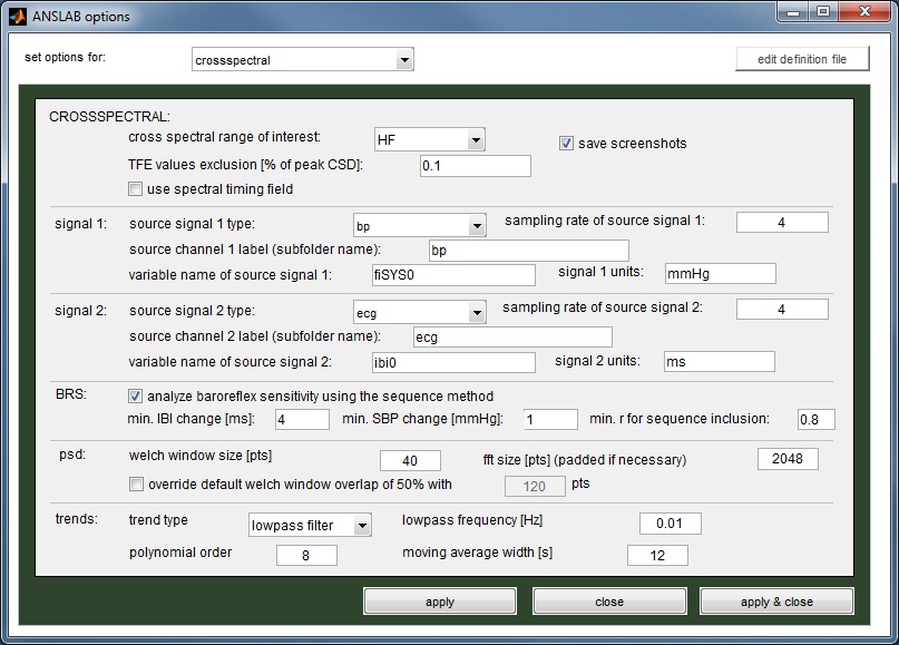
The example below uses the traces fiSYS0 (systolic blood pressure) from the blood pressure analysis and the ibi0-trace from the ecg analysis. Like in the spectral analysis, you start by selecting the raw (!) data file you wish to process. ANSLAB then looks for the specified variables in the dependent result data file in the given subfolders of the specified channel type subfolders of the study folder (so for the example below, ANSLAB will try to find the variable fiSYS0 in a data file taken from the 'bp'-subfolder in the 'bp'-subfolder and the ibi0-variable in a data file taken from the 'ecg'-subfolder in the ecg-subfolder of the selected study folder).
ANSLAB assumes that these signals are sampled with the here given sampling rates (both variables - fiSYS0 and ibi0 - are saved with 4 Hz by default).
[Top]
Timing files
Before loading the data, ANSLAB will check if a spectral-timingfile is present next to the raw datafile. If so, intervals to be processed will be taken from that file. A spectral timing file has the same structure as standard ANSLAB timing files, except that it is named 'MyFileName.spectral.m' instead of 'MyFileName.m' (see timing files for for more information).You can create such a timing file by running the marker analysis. You can additionally subdivide intervals created with the marker analysis using timing file modification from the tools menu.
Note: the timing file for crossspectral and spectral analyses are the same, as it is assumed that if both analyses are run, they will in almost all cases be run for the same intervals.
[Top]
Crossspectral analysis procedure
After opening the data file ANSLAB loads the signals, jumps to the first interval defined, and displays the signals, an underlying trend and the resulting power spectra, crossspectrum, transfer function, coherence and phase spectrum for this piece of data.RSA frequency bands are colorized, and a local maximum of the crossspectrum is identified, which is used for the extraction of transfer function, phase angle and coherence values. This maximum is plotted as a red line in the crossspectrum, and you can drag this line to an optimal position.
The band wherein the maximum is automatically searched can be set on the options dialog using the 'cross spectral range of interest'-dropdownlist. Note that when releasing the red line at a new position, tfe, coh and pha-values are updated.
Like in the spectral analysis, one can also adjust the window borders, by draging the edges of the grey surfaces to enclose only an interval of good data. When you are done, hit the accept button on the dynamic section (shown below) to go to the next segment defined in the timing file.
If an entire interval cannot be used, hit the set missing button (tfe, coh and pha are displayed as NaN) and hit accept to save the missing values and jump to the next segment. The <<<-button allows you to go 1 segment backwards, the restart button will erase all editing and begin with segment 1, and the clear segment-button will only erase editing in the current segment. Using the jump-to-segment-editbox, you can jump to a segment of your choice.

[Top]
Computing baroreflex sensitivity (BRS) using the sequence method
Starting with ANSLAB 2.6, the crossspectral method also allows to assess the baroreflex sensitivity based on the sequence method (i.e. using systolic blood pressure and IBI data).Based on the systolic blood pressure signal from a blood pressure analysis in ANSLAB and an IBI signal from an ecg analysis in ANSLAB, this method looks out for sequences of at least three consecutive rises (up-sequences) or drops (down-sequences) which are present concurrently in both signals. For a valid up-sequence (down-sequence) the rises (drops) between the successive data points must meet minimum change criteria, which can be configured in the options (see image below). These values are 4 ms and 1 mmHg for the IBI signal and the blood pressure signal, respectively.
So, if, for example, for at least three time points the difference between consecutive IBI values is at least 4 ms and if for the same time points the consecutive SBP values always differ by at least 1 mmHg, these time points constitute a valid up-sequence.
For each sequence found, ANSLAB computes a slope and a correlation coefficient. Sequences which have a minimum correlation value (default 0.8) are then used to compute the mean slope for the up-sequences and the mean slope for the down-sequences (in ms/mmHg). These values are stored along with the crossspectral analysis results and may be exported later for use in another program.
Note: the BRS analysis will be carried out for the timing file segments as specified in the respective crossspectral timing file.
To perform BRS computation based on the sequence method,
- enable BRS computation in the crossspectral options diaolog (tools -> options -> crossepctral).

- adjust the BRS parameters to suit your needs
- select 'bp' and 'ecg' as source signal types.
- enter the right subfolder names for the source channels.
- enter names of valid uniformly sampled variables (e.g. fiSYS0 for bp and ibi0 for ecg).

[Top]