Impedance cardiography
What does this channel measure?
Electrical impedance changes in the thoracic cavity are largely
dependent on the movement of blood. The largest contributor is the
blood that is pumped vigorously by the left ventricle into the aorta
with every heartbeat.
The impedance cardiography (ICG) dZ/dt signal captures the velocity changes of the blood allows estimating
pre-ejection period (PEP), left-ventricular ejection time (LVET), and stroke volume, among other cardiovascular parameters.
PEP measures the latency between the onset of electromechanical systole, and the onset
of left-ventricular ejection.
Interest in PEP springs largely from studies suggesting it is most heavily influenced by sympathetic
innervation of the heart. Particularly in combination with the parasympathetic marker of cardiovascular activity RSA, PEP can be used
to partition components of autonomic activation in a study of cardiovascular reactivity. PEP is noninvasively measured for any given
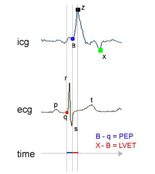
beat as the time between the Q-point in an electrocardiogram (ECG) signal and the B-point in the derived impedance signal, dZ/dt.
The B-point in the ICG represents the opening of the aortic valve, when the blood suddenly shoots out of the already contracted left ventricle
into the aorta. The B-point dZ/dt value is usually around 0, corresponding to very low velocity of the blood. The X-point represents
the closing of the aortic valve to prevent the blood from the aorta streaming back into the left ventricle. Since the direction of blood
flow at this point has typically already reversed (because of the 'cardiac afterload', the blood pressure the heart has to pump against),
the X-point dZ/dt value is usually somewhat negative. The Z-point (dZ/dtmax) represents the maximal speed of the blood ejection.
From these 3 points in relationship to the Q-point in the ECG, a variety of meaningful parameters can be estimated:
- PEP (pre-ejection period, in ms)
interval from Q-point in the ECG to the B-point in the ICG. PEP is inversely related to left-ventricular contractility and beta-adrenergic
(=sympathetic) influences on the myocard (=heart muscle).
- LVET (left-ventricular ejection time, in ms)
interval from B- to X-point in the ICG. This is how long the heart pumps blood out of the left ventricle.
- Inverse ejection-fraction index (ratio)
ratio adjusting PEP for LVET (both are highly negatively correlated with heart rate):
this is suggested to be an index of left-ventricular function that is inversely related to ejection fraction
(the percentage of blood pumped out from the left ventricle with each heart beat; compromised hearts have a lower ejection fraction).
- Peak ejection velocity index (in Ohm/sec)
this is the amplitude of the ICG Z-point (dZ/dtmax) relative to the B-point. A higher ejection velocity is produced by higher cardiac contractility.
- Heather Index (Ohm/sec2)
ratio of dZ/dtmax to Q-Z interval (electromechanical time interval). This index has been shown to be especially sensitive
to changes in cardiac contractility. Sometimes this index is adjusted by the baseline impedance (Z0) and is then measured in units of 1/sec2.
- Stroke volume (in ml)
calculated from the ICG signal using the Kubicek formula:
SV = rho * (L/Z0)2 * LVET * dZ/dtmax
where
rho = blood resistivity
L = distance between frontal ICG electrodes (in cm)
Z0 = baseline impedance displayed on the impedance cardiograph during the recording (should be stable)
LVET = left-ventricular ejection time (in sec)
dZ/dtmax = peak ejection velocity
From stroke volume, cardiac output (= heart rate * stroke volume) and total peripheral resistance (= mean blood pressure / cardiac output) can easily be computed.
[
Top]
Data preparation
Because the ICG signal is highly susceptible to even subtle movement artifacts and isometric muscular contraction near the thorax, it is typically necessary to average
the wave forms across many beats to overcome the noise confound and assure reliable detection of the B-point and other inflection points in the ICG curve.
This averaging relies on the times specified in a special ICG timing file, which has the same type as standard ANSLAB timing files, except that it is named
'MyFileName.icg.m' instead of 'MyFileName.m' (see
timing files for more information):
segments found in this file will be used for beat averaging. You can create such a timing file by running
marker analysis.
You can additionally subdivide intervals created with the marer analysis using
timing file modification
from the tools menu.
Information from the analyzed ECG file is also needed for performing averaging of the wave forms, so make sure to have run the ecg analysis beforehand.
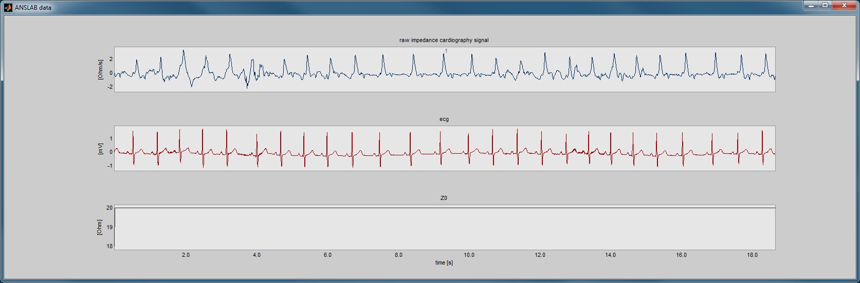
If beat averaging is not synchronized as shown in the picture below, sampling rate information that was used for ecg analysis is likely to be incorrect:
times of R-waves are interpreted based on the sampling rate information and beat epochs are extracted according to these times. Therefore,
if the ecg-sampling rate is incorrect, beat epochs are badly selected.
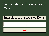
Thirdly, for each subject the main impedance level and the sensor distance is required. You can supply this information manually by entering the corresponding values
in the dialog forms shown below:

Less laborious is however to collect these values for all subjects in a textfile and have ANSLAB read the values from this textfile
automatically. This textfile must located directly in the icg-subfolder of your study folder (not in a subfolder of it) and must be called
'icgparam.txt'. This file must contain three tab delimited columns of only numbers, the first column
beeing the subject number, the second column sensor distance given in centimeters and the third the the impedance given in ohm.
An example content of 'icgparam.txt' is shown below (subject 19 - 32):
    19    15      24
    20    15      28.5
    21    8.35    21.2
    22    6.9     31
    23    14.35   28
    24    12.4    27
    25    15.75   23.6
    26    17.1    27
    27    15      30
    28    13.8    32
    29    8.25    33
    30    20.35   30.5
    31    18.15   32
    32    13.75   31
Regarding the impedance, ANSLAB also offers the option to use a channel stored in the raw file.
If this option is chosen, ANSLAB uses the mean impedance level within a segment based on the
respective channel values inside the segment (or, if beat-by-beat analysis is enabled, the mean
value of impedance values across a single beat).
Depending on the way you want to use to pass the needed information into ANSLAB, be sure to select the corresponding options in the ICG-options dialog.
[
Top]
ICG analysis options

The ICG options dialog provides various different options:
-
The main consideration is to make sure that the analysis sampling rate that was
used during the ECG analysis is set correctly. If this is not
done, the ensembles don't line up.
It is recommended to use the highest possible analysis sampling rate allowed by
the data for both ECG as well as ICG analysis (recommendation is 1000 Hz) to
achieve an appropriate effective resolution for PEP and RSA estimation.
-
For some subjects, there is no indication of any inflection in the
wave form indicative of the B-point. For these subjects, it is best to
use the zero-crossing mode across all tasks.
-
Usually the 60 Hz (50 Hz) digital notch filter should be applied to filter
out line noise.
-
If the ECG was very noisy, the Q-point detection is relatively
unstable, and it is better to estimate it by a fixed interval backward
from the R-wave peak. This interval can be set for each subject based
on an inspection of the raw ECG in exam.
-
The resistivity of the blood can change with age and during stress,
but it has been shown that under normal circumstances it can be set to
a constant value of 135 Ohm * cm in humans.
-
The stroke volume calibration factor allows to adjust the stroke
volume estimation by a constant factor. This is especially useful if a
concurrent invasive measurement of baseline stroke volume was done. In
that case, ICG derived stroke volume tracks real stroke volume during
stress very well.
Without calibration, ICG derived stroke volume can be
inaccurate on an absolute level, and thus baseline differences between
groups have to be interpreted with caution.
-
Usually taking the median across the ensembles is more accurate than
the mean, because outliers are given less weight.
-
The ICG wave form display window can be adjusted to provide optimal
resolution for judging the location of the B- and X-points. Especially
for subjects with very high baseline heart rates this can be made
smaller, e.g., 500 ms.
-
In many subjects there is a double-trough in the area where the
X-point is expected. With some judgment (see also below), you can
decide which one represents the closing of the aortic valve. This
decision then has to be applied to all tasks for this subject.
ANSLAB allows to setup a search mask for detection of the correct
X-point. This detection window is used in case of an ensemble analysis
as well as in case of a beat-by-beat analysis.
-
The detection algorithm for the B-point looks for an inflection point
somewhere in the area before the steepest increase in the ICG signal
occurring before the Z-point. Some subjects have pronounced inflection
points, others have barely visible ones. ANSLAB allows to
adjust the sensitivity of this detection. In addition, ANSLAB allows to switch
to another detection method (i.e. the zero-crossing method), which uses the
time point of the zero crossing before and closest to the z-point.
If the detection is set to 'notch' and ANSLAB is not able to find a valid B-point, the user is asked whether the zero crossing method
should be used as a fallback solution (in batch mode this is done automatically).
-
ANSLAB allows to specify the minimum number of beats per segment required in order
to regard a segment as a valid one. If the number of beats detected in a segment
lies below that value, the ICG export parameters for that segment are set to missing (i.e. NaN values).
[
Top]
Analysis procedure
Segment-based vs. beat-by-beat analysis
Starting with ANSLAB 2.4, you can choose to either perform the ICG analysis
based on timing file segments, on a beat-by-beat basis, or both (the analysis mode can be set
in the options).
- Segment-based analysis
In this mode an averaged ICG waveform is computed from all heart beats detected within a segment
in the timing file. This mode is usually more reliable since outliers are given less weight. But the temporal resolution
is rather low (depends on the length of the segments provided in the timing file).
- Beat-by-beat analysis
ANSLAB also allows too run an ICG analysis on every single beat, having ANSLAB find the B-, Z- and X-point automatically
(to activate the beat-by-beat analysis, set the "analysis mode" dropdown box on the ICG-options page to "both" or "beat-by-beat").
This gives you better temporal resolution, but accuracy of the calculated parameters depends much more on the signal quality.
After the beat-analysis, the calculated parameters are displayed (as shown below) and you can edit the calculated parameters for outliers
using the exclude editing tool. If both the segment and the beat-by-beat analysis are run, beats excluded in the segment analysis will
automatically be set to missing in the beat-by-beat analysis.
Considerations for batch mode
The ICG analysis may also be run in batch mode. However, since there may be high inter-subject differences with respect to
the location of the characteristic points in the ICG waveform (i.e. B-, Z-, and X-point) it is recommended to
carry out a manual analysis.
This is especially true in cases where the ICG signal has a low signal quality. In such a case it is crucial to set
the detection windows right. You may run a batch analysis in this case, followed by batch plotting and make a judgement
on the right detection windows for all subjects.
[
Top]
Editing of ICG data
As with the other variables, select the file you want to look at. ANSLAB preprocesses the dZ/dt signal and in the first display (axis A) shows the dZ/dt ensembles
synchronized by the ECG Q-point of each heart beat. In the second axis, an ensemble average across the shown beats is displayed, with standard error
margins and the automatically detected B-, Z-, and X-point, as shown below.

You can display the corresponding piece of raw signal by selecting the 'see raw signal' button:
Outlier exclusion and autoexclusion
You can manually exclude outlier curves using the 'exlusion box' outlier rectangular function in the left axis.
Moreover, if autoediting is activated in the ICG options, ANSLAB automatically exludes outlier curves that are above or below the mean +/- 2 standard
deviations in the B-point window (shaded in light red).
Special emphasis is put on the B-point window, as outliers distort this point most heavily, although you can extend the sensitive window to cover the
entire beat. Exluded curves are plotted in light red. You can adjust the auto-editing parameters (sensitive window and standard deviations
factor) in the ICG-options. The auto-editing outlier criterion is calculated statically using all beats in a segment, whereas the +/-1 standard deviation range in the
average plot is updated automatically based on remaining valid beats. Hitting the 'clear seg'-button will undo all exclusions for the current segment
(including auto-exclusions).
Adjusting the B-, Z- and X point
You can drag the B-, Z,- and X-point in the right axis. You can also drag the detection windows. Dragging the
left line of a detection window will move the window to a new position. Dragging the right line allows to change the window size.
Number of beats, number of excluded beats, segment number, PEP and LVET values are displayed and updated according to editing steps in the data window.
The detection window positions and widths are also shown in the dynamic section and can be changed by entering new values (values are given in milliseconds and
relative to the Q point position).
The detection window settings can be saved for use with other files by pressing the 'save'-button.
Selecting a point (X, Z or B) with the mouse also activates that point for a precise adjustment with the
arrow keys (left and right). This is indicated by the 'arrow key setting active for:'-radiobuttons:
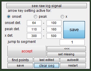
The activated option shows which point can be moved by pressing the left and right arrow key. Using this option, the points are moved by a very
small amount (1 ms per keystroke). Therefore, adjusting the points roughly with dragging first is advisable. ANSLAB will remember
exluded beats for a segment and point position changes you performed with dragging. If you whish to reset these choices for a given
segment, press the 'clear segment'-button. Pressing the 'clear all'-button will reset all editing steps performed so far and restart with the
first defined segment.
Pressing 'accept' will save the current averaged waveform along with the the B-, Z- and X-points and continue with loading the beats of the next
segment. You can set a segment to missing data by choosing the 'set missing'-button. Hitting the '<<<'-button allows you to go back to the
previous segment and continue editing there. You can also jump to a segment of your choice by entering a number in the 'jump to segment'-editbox, and you
can save editing results to the current point by hitting the small 'save'-button.
If loading of previous analysis results is activated in the ICG options, these editing results are loaded when reopening the file
for analysis. You can then use the 'last edited'-button to jump to last segment for which editing results can be found. After the all segments have been
processed, extracted parameters are plotted over the duration of the file and you can choose to save the reduced data to file or discard analysis
results. Note that extracted calculated traces are plotted as 'event'-type traces and can be directly aligned and compared with raw
ICG and ECG signal by switching from 'event' to 'raw'-display-mode.
[
Top]
Guidelines for setting characteristic points
The Z-point is almost always easy to identify and the detection algorithm hardly makes a mistake here. The B- and X-points can be more
problematic in some subjects during certain tasks, especially if there is much movement artifact. And of course, analyzing ICG is much easier
in young and healthy subjects than in older adults with cardiac disease.
If you see a distinct B-point in the raw data but not in the ensemble average this indicates that the ensembles are not aligned well
and that the inflection point is 'washed out'. This could be because of a noisy ECG resulting in errors in the Q-point detection (in the order of a few
milliseconds). But the Q-point times are the basis for the alignment of the ICG ensembles. If you are facing this problem you could use enable
the option to use the q_fixed Q-point estimation. This forces ANSLAB to align the ICG at a Q-point estimated from the more reliable R-waves.
Another reason could be that the period you are averaging over does not represent a steady state. If the PEP changes considerably across your
averaging period, this would also wash out the B-point inflection from the ensembles. In this case it is recommended that you define smaller
segments in the ICG timing files. A reasonable estimation of ICG parameters can be based on as few as 15 beats. Note that PEP and other ICG parameters depend to some degree
on the filling of the lungs, so it is important to average across several breaths.
If you can not see a distinct B-point in both the ensemble averages and raw data, this indicates that the subject has a cardiac and thoracic
morphology that makes estimation of PEP with just spot electrodes difficult. You could exclude this subject from the ICG statistics or
use the zero crossing mode. You may also manually reset the B-point to the zero dZ/dt line. This needs to be done across all tasks to be consistent.
The X-point can sometimes be ambiguous. There can be two or even three dips after the peak in the ICG signal. As a general rule it is then
the second or third dip. Among these two it is the one followed by a consistently steeper immediate increase, which indicates the closing of the aortic
valve and sudden stop of reflux of blood into the left ventricle. Another guideline is that typical LVET values for young healthy subjects range between
300 and 350 ms, but it also depends much on various factors like physical fitness and body mass index. It is important to be consistent with the
identification of the X-point within subjects.
Sometimes excluding a problematic subject from the analysis of ICG derived parameters is the best option and helps to not distort group
statistics.
[
Top]