Reflexive startle electromyography

What Does This Channel Measure?

People exhibit in response to a sudden threatening event a whole body startle response, including increased heart rate, contraction of the neck muscles, and an eyeblink, among others. Measuring the startle response is important in the context of emotion research, as its magnitude is modulated by affective valence. Roughly, the more negative someone feels the larger the magnitude of the startle response. Typically, startle responses are provoked using loud (95 dB), sudden (50 ms) bursts of white noise – so-called startle probes. As an indicator of startle magnitude we use the strength of the eyeblink response, which is measured with electromyographic (EMG) activation of the lower eyelid. anslab preprocesses and displays this EMG activation and allows to edit it for individual startle probes.

analyzing startle data:

Starting with anslab2.4, there are two different ways of analyzing startle data:

1) The raw data file contains a marker channel that indicates when the startle probe was given ("channel").
2) The timepoints of the startle probes are given in a timing file ("timingfile").

You have to specify either "channel" or "timingfile" in the startle options, using the marker type dropdown box. For the case of a marker channel, the marker needs to go up when the noise burst starts and down when the noise burst ends. After loading the data file containing the EMG- and the marker-signal, you are prompted for this threshold:

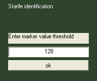
Every timepoint  the marker channel rises above this threshold is considered to be the onset of a startle tone. For the case of timing files, startle onsets are taken from an associated timingfile. All entries in the timing files are considered as startle trials independant of the segment value.

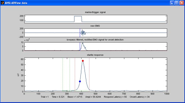
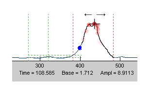
Next,  the first startle probe (=trial) is displayed. Examples of this are shown below.  Here’s how to read the startle data display window:

• first graph, dark blue line = trigger signal
  
• second graph, dark blue line = raw emg
  
• third graph dark blue line = rectified and lowpassfiltered EMG signal used for onset detection
  
• fourth graph, dark blue line = filtered and rectified EMG signal for startle amplitude measurement (this is what you should focus on)
• fourth graph, first vertical green line = start of baseline
  
• fourth graph, second vertical green line = probe onset and end of baseline
  
• fourth graph, lower horizontal green line = startle response baseline value (average of the baseline window)
  
• fourth graph, higher horizontal green line = indicator for 5 standard deviations of signal within baseline window above the average baseline
  
• fourth graph, red area = startle scoring area (anslab only looks for a response in the window between 20 and 120 ms after the startle probe as this is physiologically the time window a startle response is expected to occur. Sometimes there will be a second, partially voluntary response, after this time window which we do not want to include).
• fourth graph, red dot = marker for detected response maximum and response latency
• fourth graph, blue dot = marker for response onset (derived from third graph)

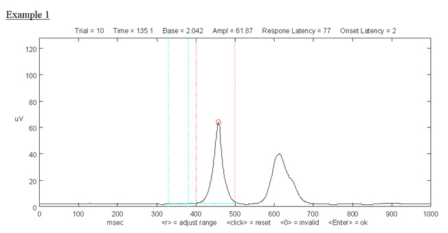
adjustment of automatic detection parameters:   In the example below, the baseline interval and the response window are not adequate for the data: the baseline window covers part of the response and the response window misses the response's maximum.

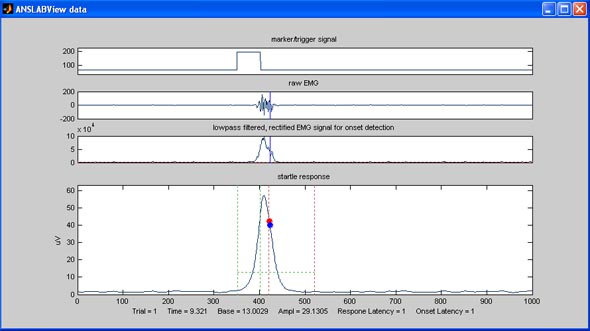
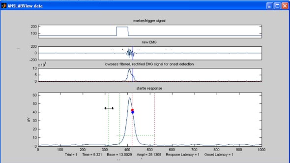
The correct timing of the baseline and response window depends very much on the actual triggering- and sound-display-hardware, it is therefore quite often necessary to shift both windows to fit your setup. This is no problem, as long as you keep these parameters constant over all your trials.  To shift either the baseline or the response window, you can drag-and-drop the dotted lines on the graph to an optimal position:

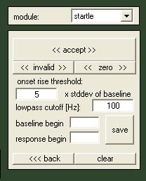
The response onset latency is identified using the third graph, that shows a lowpass filtered rectified emg signal. An onset is detected, if the curve rises above a the mean value during the baseline interval plus a customizable number of standard deviations of the baseline signal. This threshold is illustrated by the horizontal red line in the third graph.  You can adjust the threshold, by using the 'x stddev of baseline'-field in the startle-control-section of the command window.  In the example below, this threshold was clearly chosen too large, the onset time beeing overestimated:

You can also modify the cutoff-frequency of the lowpass filter, that is applied to this onset-detection-signal, by changing the value in the 'lowpass cutoff []Hz]'-field.

Note that when setting the analysis type to 'startle', the 'dynamic'-section switched to show the startle scoring controls. When you drag and drop the response window to an optimal position, the position of these windows are updated in the 'baseline begin'- und 'response begin'-field  of the startle control section, shown below. To save these position and the currently set onset threshold factor and cutoff-frequency for use with other files, simple hit the save button. The values are saved in your 'anslabdef.m'-file in the study folder.

scoring startle trials : You use the accept-, invalid- and zero button,  to jump from trial to trial and decide wether trials are valid or not. 'Accept' will save the current trial and jump to the next. 'Invalid' will set parameters for the current trial to NaN (not a number), 'zero' will set them to zero. The extracted variables are displayed in the command window. This output could look like this:

You can see that five variables are extracted for each startle response, sa (startle magnitude), sb (startle baseline level), st (the abolsute time of the response),  so (startle onset latency) and sl (startle response latency).

Most important of these are startle response magnitude (=peak minus baseline value), startle response latency (from tone onset to peak response as evident in the EMG average upper window), and startle onset latency (from tone onset to onset of EMG response as evident in the upper raw EMG window). These variables are illustrated by the red and blue dot in the startle response graph. If the automatically set positions of these dots do not seem appropriate to you, you can drag and drop the dots to a position along the response line - latency and magnitude values will be updated according to the new positions.

setting the startle response maximum:  If there are two equally plausible peaks pick the one closer to the normal response time for that subject and above the 5 SD line [see Example 2 below --> the first response is closer to this subject’s  normal response latency].  If there is no clear response, move the dot to a clearly identifiable peak that is approximately at the normal response time for that subject in order not to distort response latency. Do this only if the standard deviation is low. [See example 3 below --> this response might justifiably be set a little later on the second discernible peak if it reflects the subject’s normal response latency; or alternatively, set to 0 response.]  If the standard deviation is higher (i.e., much higher than any of the responses in that trial), consider excluding this response by hitting the  'invalid'-button, as this response measurement is probably not reliable due to an instable baseline.      

The response onset latency is marked with a blue dot. You can drag this marker just like the maximum response marker.

After you have gone through one file trial-by-trial, startle magnitude and latencies are displayed for each response. They appear as step functions, because anslab is set to extrapolate from each response for the whole intertrial interval. Choose 'save reduced' to save response scores to disk: both, a mat-file and a text file are created in the startle subfolder of your study folder.

Text output of Startle Data:

This is an example of a textfile written by anslab after the analysis of each file:

Trial    Time           Amplitude    Latency   OnsetLatency  BaselineAmplitude    Condition
1        198.195        7.2207       106       63            4.9394        132
2        204.252        7.484        78        59            6.9037        132
3        212.312        41.4574      84        62            4.9877        132
4        221.371        34.3716      77        55            4.824         132
5        226.427        13.4875      82        68            4.6159        132
6        236.478        40.224       66        46            5.39          132
7        320.123        24.1213      84        56            4.2921        136
8        327.174        18.515       81        57            4.8101        136
9        339.225        4.4587       68        53            3.9588        136
10       356.273        39.9746      67        43            3.8594        136
11       368.317        12.6836      66        52            4.9739        136
12       375.37          6.0252       85        60            4.5096        136
13       384.43         -9999        -9999    -9999          8.4283        136
14       398.48         12.6606      70        57            4.6539        136
15       408.524        9.2906       68        55            5.089         136

Times is given in seconds since file begin, the response Amplitude is already baseline corrected (so the non-baseline corrected response amplitude can be obtained by adding BaselineAmplitude to Amplitude), Latencies are given in milliseconds. Condition refers to the marker value recorded at the presentation of the startle tone. Missing data is stored as -9999.

Mat output of Startle Data:

Here’s what the variable names in the text-file mean:

Ratio adjustment for reactivity scores (task minus baseline) may be more appropriate than change scores with EMG data. The startle response magnitude for a given individual depends on many factors: exact placement of the electrodes, muscle size, innervation density, skin thickness, etc. All these are probably multiplicative rather than additive factors for the response estimation. However, often additive change scores are used in publications.

Editing Examples: